Creating Mandelbrot and Julia Set Fractals

When I first started playing around with fractals many years ago it was difficult to find a simple concise description of how Mandelbrot and Julia sets were constructed. I had to put the story together with details from various web sites and books, so I thought I would make it convenient for others by describing the process here. The following discussion covers the escape time algorithm which is somewhat limited in the number of colors it can produce but it’s a good place to start. Later several variations are mentioned that can produce smoother images with a much broader color range. There is also a list of references for more information at the bottom of the page. This discussion just covers how to generate the images and does not do justice to Chaos theory or Fractal geometry. For a deeper understanding of the theory please check out the references.

Since these algorithms are based on complex numbers let’s start off with a review of some of the basic math. Complex numbers consist of a real and imaginary component. For example consider the complex number z below, which has a real number component x and an imaginary number component yi.

Imaginary numbers are a mathematical invention to account for the problem of taking the square root of a negative number. Imaginary numbers include the letter i as a factor to represent the square root of -1.

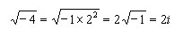
For example, to obtain the square root of a negative number, the i can be factored out.

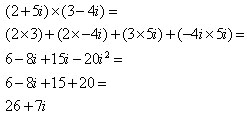
In the equation above, the y factor of yi is a real number just like x. Complex numbers can be manipulated like binary numbers with special attention given to the factor i. Operations on complex numbers usually result in a complex number. For example consider the multiplication of the two complex numbers below.

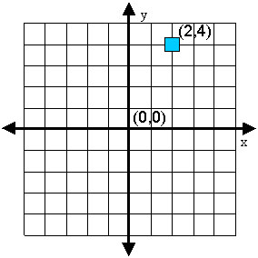
The real and imaginary components of complex numbers can be used to represent different dimensions. For example, complex numbers can be plotted on the Cartesian plane with the real component along the x-axis and the imaginary component along the y-axis. The following figure shows the complex number z = 2+4i plotted on the Cartesian plane.

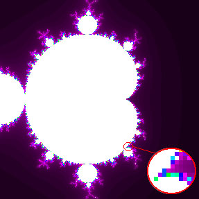
Cartesian coordinates can also be used to represent location on a computer screen. Computer images are composed of numerous small squares called pixels. Each pixel displays a single color at a given moment. When magnified, a computer image looks like a mosaic of colored tiles. However when viewed as intended, the eye perceives the image as a smooth continuous picture. The image below shows a Mandelbrot set with an enlargement of a small area demonstrating the mosaic appearance of pixels.

Mandelbrot and Julia set fractals are constructed using functions of complex numbers. One of the simplest and most commonly used functions is:

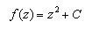
Where both z and C are complex numbers. This is the equation used to generate the preceding Mandelbrot set image. Where:

When calculating Julia sets, z is a variable representing a Cartesian coordinate within the image and C is a constant complex number. C does not change during the calculation of the entire image. However, when different values of C are used, different images representing different Julia sets will result.

The first step to calculate the image is to choose an equation and a value for the complex constant C and then plug a screen coordinate value (x,y) into z. The ultimate outcome will be to assign a color to the pixel that maps to the given (x,y) coordinate. Notice that I said first step. The output of the function f(z) is not used directly to determine the color of a given pixel but it is the start of the process.

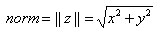
The second step is to calculate the norm or size of the result of f(z). Processing the function f(z) on the given values of z and C yields another complex number. The norm of this number is calculated using the equation below. The value of the norm will be a real positive number. The value of the norm is then compared to another number called the bailout or blowup number. If the value of the norm is greater than the bailout parameter a value of zero is assigned to the pixel. Otherwise if the norm is less than or equal to the bailout number, the value of f(z) will be substituted back into the equation as the next value of z. Next the norm of f(z) is again calculated and compared to the bailout parameter. This time if the norm is greater than the bailout parameter a value of 1 is assigned to the pixel, but if it is not, the new value of f(z) is substituted back into the equation in the place of z. This process is repeated over and over until the norm is greater than the bailout parameter or the number of cycles or iterations exceeds some maximum number. The number of iterations that have occurred until the norm exceeds the bailout parameter will be used to assign a color to the pixel. The number assigned to the pixel will be an integer value between zero and the maximum number of colors used to make the image.

The series of calculated values for a single point in the Mandelbrot or Julia set is referred to as an orbit. Orbits can exhibit different behavior. Some orbits tend to move towards a fixed number, some oscillate back and forth between values, and others escape to infinity. The orbit is compared to the bailout number to determine if it will escape. In this coloring algorithm, the colors are determined by how fast the orbit escapes.

Finally the process just described for a single pixel is performed on every pixel in the image, one pixel at a time.

Typically the maximum number of colors using this algorithm is 256. Each integer will represent a different color and these will be linked in some kind of table or palette. For example a value of zero may represent black, one could be violet, and two could be red, and so on. Many image formats or file types like bitmaps store an image as an array of integers representing the pixels and a color table, which tells the computer which color to map to the indexes in the image array.

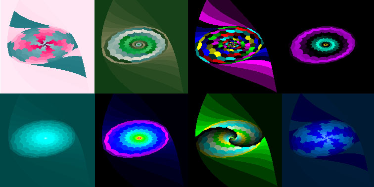
The colors used in the table or palette can have a big effect on the way an image appears. In the figure below, each image has the same integer values assigned to all the same pixels but the color table has been changed.

The calculation of a Mandelbrot set is similar. The difference is in the values that are substituted into the equation. In the equation for f(z) the pixel coordinate (x,y) is substituted into the complex number C and (0,0) is substituted for a starting value of z. After the first iteration, the value of f(z) is substituted for z just like when calculating the Julia set.

As mentioned earlier the escape time algorithm results in images with a limited number of colors and typically the images appear to have color bands or stripes. While these can be interesting many people find it more aesthetically pleasing to produce images with more colors that produce smoother gradients. One method to produce such images is e^-|z| smoothing. Instead of calculating the norm and comparing it to a bailout number the value of e^-|z| is calculated at each iteration and summed over all iterations. Another method for producing smoother fractals is the Distance Estimate method. The distance method involves calculating the following formula for each point.

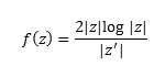
Where z’ is the derivative of z and |z| is the norm of z

Another coloring algorithm that deserves mention is orbit traps. This is actually a group of related methods that involve calculating the distance between some region in complex space and z.

Reference

Peitgen, Heinz-Otto, Jurgens, Hartmut, and Saupe, Dietmar (2004). Chaos and Fractals: New Frontiers of Science. New York Springer-Verlag New York Inc. This book covers a broad range of topics. The theory and math is explained at a level that is comfortable for a broad range of readers. Anyone really interested in fractals should check this out.

Mandelbrot, Benoit D. (1982). The Fractal Nature Geometry of Nature. W.H. Freeman and Company. This is a classic by the father of Fractals.

Devaney, Robert L.(1990). Chaos, Fractals, and Dynamics. Addison-Wesley Publishing Co. A good beginner book to learn the theory with example BASIC programs.

Gleick, James (1987). Chaos: Making a New Science. Viking Penguin. Casual reading history of Chaos and Fractals.

Fractal Coloring Algorithm Links

Coloring Dynamical Systems in the Complex Plane

Orbit Traps